

Abstract
Current understanding of the cold season Arctic oscillation (AO) impact on the summertime sea ice is revisited in this study by analyzing the role from each month. Earlier studies examined the prolonged AO impact using a smooth average over 1–2 seasons (e.g. December–March, December–April, March–May), ignoring large month-to-month AO variability. This study finds that the March AO is most influential on the summertime sea ice loss. First, the March AO is most highly negative-correlated with the AO in summer. Secondly, surface energy budget, sea level pressure, and low-tropospheric circulation exhibit that their time-lagged responses to the positive (negative) phase of the March AO grow with time, transitioning to the patterns associated with the negative (positive) phase of the AO that induces sea ice decrease (increase) in summer. Time evolution of the surface energy budget explains the growth of the sea ice concentration anomaly in summer, and a warming-to-cooling transition in October. The regional difference in sea ice anomaly distribution can be also explained by circulation and surface energy budget patterns. The sea ice concentration along the pan-Arctic including the Laptev, East Siberian, Chukchi, and Beaufort Sea decreases (increases) in summer in response to the positive (negative) phase of the March AO, while the sea ice to the northeast of Greenland increases (decreases). This sea ice response is better represented by the March AO than by the seasonally averaged winter AO, suggesting that the March AO can play more significant role. This study also finds that the sea ice decrease in response to the positive AO is distinctively smaller in the 20th century than in the 21st century, along with the opposite sea ice response over the Canada Basin due to circulation difference between the two periods.
Export citation and abstract BibTeX RIS

Original content from this work may be used under the terms of the Creative Commons Attribution 4.0 license. Any further distribution of this work must maintain attribution to the author(s) and the title of the work, journal citation and DOI.
1. Introduction
The Arctic oscillation (AO) in the boreal winter significantly explained by natural variability (Screen et al 2018) is understood as one of the key factors for driving the anomalous surface condition in the following melt season (Rigor and Wallace 2004, Lindsay and Zhang 2005, Kwok 2009, Polyakov et al 2012, Döscher et al 2014). Earlier studies showed that the wintertime AO can have persisting impacts on the surface temperature, pressure, sea ice drift and circulation in the subsequent months. Most importantly, this memory of the wintertime AO can play a profound role in driving variability of the summertime sea ice (Rigor et al 2002, Zhang 2015, Ogi et al 2016, Park et al 2018, Gregory et al 2022). Rigor et al (2002) and Williams et al (2016) found that sea ice motion that responds to the positive phase of the AO modulates the Beaufort Gyre, Transpolar Drift Stream (Mysak 2001) and subsequent ice export through the Fram Strait (Ogi and Wallace 2012), enhancing the summer sea ice loss. Several studies attributed this ice export to the Arctic dipole pattern (Lindsay et al 2009, Overland et al 2012, Choi et al 2019). In contrast, Beaufort Gyre was found to be stronger after the negative phase of the winter AO leading to thickening of the sea ice pronouncedly in the Canada Basin (Proshutinsky and Johnson 1997). Atmospheric circulation and surface radiative/turbulent heat fluxes in spring and summer can be also modulated by the AO forcing in the preceding winter (Park et al 2018). Williams et al (2016) used a hindcast model based on the AO index averaged over winter and spring (December–April) and was able to reduce errors in anticipating the sea ice extent anomaly in September.
In addition to the wintertime AO impact, studies also found that the sea ice extent minimum in late summer (August–September) is highly correlated with reflectivity of solar radiation in early summer (May–June) (Choi et al 2014, Zhan and Davies 2017). Kapsch et al (2019) addressed a key role of spring atmospheric circulation patterns in modulating the Arctic sea ice in summer.
Different conclusions from earlier studies indicate that there is still room for further improved understanding of time-lagged connection between AO and sea ice. Advanced understanding is also expected to contribute to the improvement in seasonal prediction skill of the summertime sea ice. Currently, many climate models such as the ones participating in the Coupled Model Intercomparison Project 6 (CMIP6) have underestimated the important connections between the winter AO (average over December through March) and the summer sea ice (Gregory et al 2022) more specifically over the pan-Arctic region such as the Laptev, East Siberian and Beaufort seas, where the strong downward trend of sea ice extent due to climate change (Meredith et al 2019) and increasing role of ocean-air heat exchange (Laptev Sea) (Ivanov et al 2019) was reported. Earlier version of climate models (e.g. CMIP5) also underestimates the observed relationship between solar radiation in early summer and sea ice extent in late summer (Choi et al 2014). Sea ice variation by atmospheric circulation associated with internal variability also tends to be underestimated (Shen et al 2022).
Although it is a common analysis to evaluate AO impacts using 1–2 seasonal average, the AO phase can vary from weekly to intra-seasonal time scale. It is not unusual to see several phase transitions and resulting changes in weather events (Rudeva and Simmonds 2021) within a season. Because of these variabilities at shorter time scales, the strongest impactful AO signal might be substantially reduced by the seasonal averaging. Thus, if the AO from each winter month has different influence on the summer sea ice, an interesting question would be: what month of the AO has the most impact?
In this study, we find that the most impactful AO is not from the winter months average. It is the March AO that produces the strongest time-lagged response of the summertime sea ice in the Arctic than all winter or winter–spring averaged AOs. This study is organized by first confirming the negative relationship of the AO phase in winter with that in the following summer (Ogi et al 2016) and extending the correlation analysis for the AOs from each individual months. Then, investigations are made to better understand how the time-lagged responses of thermodynamic (i.e. surface warming/cooling from surface energy budget) and dynamic (low-level circulation and pressure) process to the March AO evolves with time from March through September to drive the sea ice anomaly during the melt season. Finally, sea ice responses to the AO in the 21st century and the late 20th century are compared to quantify their differences (Gregory et al 2022).
2. Data and method
2.1. Data
Monthly AO index based on the empirical orthogonal function (EOF) of 1000 hPa geopotential height is obtained from national oceanic and atmospheric administration (NOAA) over the period 1980–2021. Reanalysis variables for analysis are obtained from the Modern-Era Retrospective analysis for Research and Applications, version 2 (MERRA-2) (Gelaro et al 2017). The variables used are geopotential height at each pressure level from 1000 hPa to 100 hPa, sea level pressure (SLP) and horizontal winds at 925 hPa level (GMAO 2015a), sea ice fraction (GMAO 2015b), surface shortwave and longwave radiative fluxes, latent heat flux and sensible heat flux (GMAO 2015c). Since the MERRA-2 has some limitation in accurately representing the observed sea ice distribution (e.g. warm bias in sea ice representation (Batrak and Müller 2019, Marquardt Collow et al 2020)), results from the MERRA-2 are verified by the observation from the National Snow and Ice Data Center (NSIDC) (Walsh et al 2019). Also, the surface radiative fluxes from the Clouds and the Earth's Radiant Energy System (CERES) Energy Balanced and Filled (EBAF) (NASA/LARC/SD/ASCE 2019) are used to compare the radiative fluxes between the MERRA-2 and CERES-EBAF_Ed4.1.
2.2. Method
Time-lag correlation and regression are the main methods to explore the responses of the sea ice and key atmospheric/surface variables to the AO. The sea ice and AO time series are detrended by least square estimate to remove any contribution from trend to time-lag correlations. The correlations are computed using the Pearson correlation method. To assess the significance, critical value of the correlation at 95% confidence is obtained based on the t-test with N − 2 degree of freedom, where N is the sample size. In order to identify the time evolution of the sea ice, surface warming from surface energy budget, SLP and circulation in response to the March AO, we regress their anomaly time series at each grid point onto the AO index. This regression is also applied to three-dimensional geopotential height anomalies from 1000 hPa to 100 hPa levels to acquire their vertical structure in the Arctic connected with the AO in target month that varies from December to May. A two-tailed t-test is conducted to test the significance of the regressed anomalies.
3. Results
The first step of our diagnostics is to find the cold season month in which the AO has the strongest lagged correlation with the AO in subsequent summer months. To identify that month, geopotential height anomalies in each calendar month are regressed for each pressure level onto the NOAA AO index for January (figure 1(a)), February (figure 1(b)), and March (figure 1(c)), respectively, followed by averaging the regressed anomalies over 0°–360° E, 60°–90° N. Since the loadings of the positive AO EOF are negative over this Arctic domain, the negative (positive) anomalies in figure 1 can be thought of as the positive (negative) AO phase. The vertical structures exhibit different time-lagged relationship of geopotential height with the AO in three different preceding months. Geopotential height anomalies in response to the March AO are evidently positive in summer, indicating reversal of the AO phase (i.e. positive in March to negative phase in summer) (figure 1(c)) (Ogi et al 2016). Cases for January and February also exhibit the weakening of the negative anomalies in summer (figures 1(a) and (b)), but the reversal of AO phase is not as clear as the case for March. We also compute correlation of the AO index in summer (June–September) with that from January, February, and March, respectively. Correlations turn out to be −0.08 (January), −0.10 (February), and −0.38 (March), with the largest amplitude from March. Especially, AO in August, out of the summer months of June–September, is most negatively correlated with the March AO, with correlation −0.54. Additional examination of the time-lagged geopotential height response to the AO in another months, December or two spring months (April and May), presents no clear relationship in the AO phase between those months and following summer (see supplementary figure S1). The results overall support the argument that the March AO is the most influential factor that leads to the opposite phase of the AO in the following summer. This advances the previous understanding about connection of the AO with the sea ice in summer based on the seasonally averaged AO in the preceding winter (Rigor et al 2002, Ogi et al 2016). An important finding in Ogi et al (2016) based on the seasonally averaged AO is that the September sea ice response to the AO is relatively weaker after 2007 and the surface air temperatures over the East Siberian, Chukchi, and Beaufort Seas play a stronger role in sea ice coverage in fall.
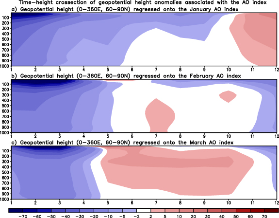
Figure 1. Time–height cross-section of the area-averaged (0°–360° E, 60°–90° N) geopotential height anomaly projected onto the Arctic oscillation index in January (upper), February (middle), and March (lower). The regressed anomalies significant at 90% confidence are shaded. Time axis represents the months in number and the vertical axis represents the pressure levels in hPa. Unit of the anomaly is m.
Download figure:
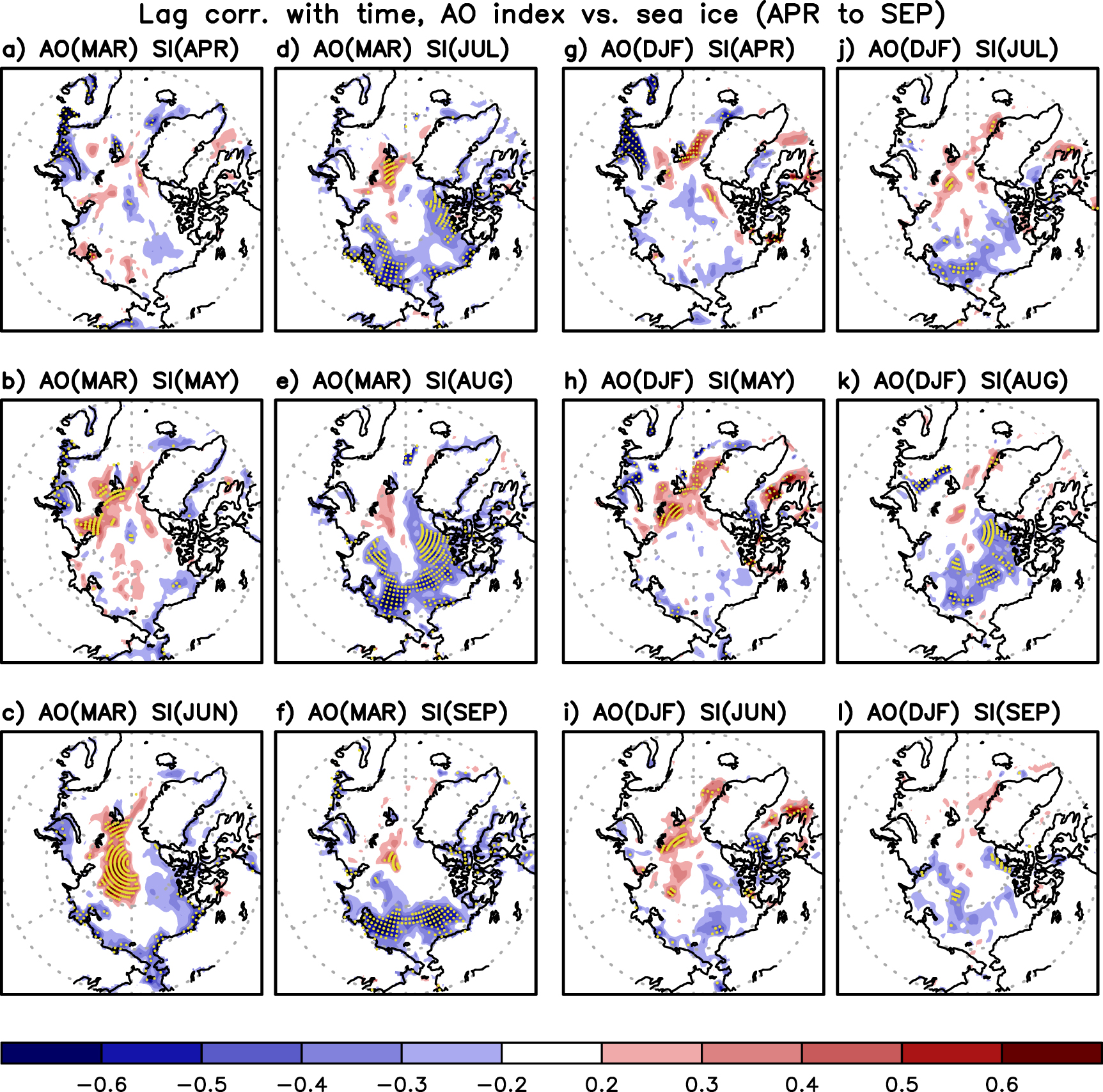
Standard image High-resolution imageThe sea ice response to the AO evolves with time, showing that regional sea ice responses are better represented by the March AO than by the seasonally averaged winter AO. The main feature revealed from lag-correlation between sea ice and March AO is that negative correlations are gradually getting stronger, signifying the sea ice decrease with time over the Laptev, East Siberian, Chukchi, and Beaufort Sea (LECB) in the event of positive AO in March (figures 2(a)–(f)) (Gregory et al 2022). The area of sea ice reduction also expands with time, reaching the maximum spatial extent in August. The strongest negative correlations (<−0.6) are seen in August, consistent with the strongest negative relationship in the AO phase between March and August (figure 1). The region of sea ice decrease shrinks to some extent in September, but the negative correlations over the LECB region remain high. In contrast, the region to the northeast of Greenland is characterized by positive correlations that indicate sea ice increase, with the maximum in June. Time-lagged correlations of the sea ice with the December, January, and February (DJF) averaged AO in figures 2(g)–(l) exhibit relatively smaller amplitudes than those in figures 2(a)–(f) (March AO) more clearly during the melting period of July, August and September.

Figure 2. (a)–(f) Time-lag correlation coefficients of the March AO index in the 21st century (2000–2021) with the sea ice anomaly for the following months of (a) April, (b) May, (c) June, (d) July, (e) August and (f) September. (g)–(l) Same as (a)–(f) but for the AO index averaged over December through February (with no impact from March). Stippling represents the grid points where correlation is significant at 95% confidence.
Download figure:
Standard image High-resolution imageThere is clear evidence that the sea ice response to the March AO is remarkably different between the 21st and the late 20th century (e.g. 1980–1999). The result for the 20th century demonstrates that the sea ice decrease over the East Siberian Sea is apparently smaller than that in the 21st century especially in climatologically a stronger melting period of August and September (figures 2(c)–(f) and 3). Sea ice in the 20th century is relatively thicker, older and more rigid, making the sea ice response to the AO less sensitive and harder to occur (Maslanik et al 2007). Particularly, the sea ice response, characterized by increase over the Canada Basin, is opposite to that in the 21st century. Not only the different nature of sea ice between the two periods, but also the different atmospheric circulation response to the AO, that will be discussed in figure 7, appears responsible for this opposite sea ice response. Also, the negative relationship of the AO phase between March and summer (August for example) in the 20th century is not as strong as that in the 21st century (Yamazaki et al 2019). The correlation of the AO between March and August is 0.10 in the 20th century while it was −0.54 in the 21st century.

Figure 3. Time-lag correlation coefficients of the March AO index in the 20th century (1980–1999) with the sea ice anomaly for the following months of (a) June, (b) July, (c) August and (d) September. Stippling represents the grid points where correlation is significant at 95% confidence.
Download figure:
Standard image High-resolution imageThe sea ice data used in figures 2 and 3 are from reanalysis. Thus, the same calculation is conducted using the observed sea ice concentration from the NSIDC to verify the reliability of the results in figures 2 and 3. The main features found in figures 2 and 3 that (a) the March AO better explains the time-lagged sea ice response in the following summer than the DJF averaged AO, (b) the largest negative correlations over the LECB region in August and September, and (c) the opposite sea ice response between the 20th and 21st century to the AO over the Canada basin, are reproduced well based on the NSIDC data (figures S2 and S3), demonstrating the reliability of the patterns in figures 2 and 3.
To better understand how the thermodynamic processes influence the sea ice response, we analyze surface energy budget. The surface energy budget is broken down, as in the following, into the net radiative fluxes and turbulent heat fluxes with the positive (negative) budget value for warming (cooling) the surface,

Time evolution of the energy budget in response to the positive March AO reveals that the Arctic Ocean is dominated by surface warming due to energy surplus (figure 4). Surface warming grows from April through August reaching the maximum in August, followed by moderate weakening in September. The surface warming is even greater along the LECB region. In contrast, east and northeast of Greenland shows surface cooling in general from May to August. This regional distribution each month is quite similar to the patterns shown in figure 2, demonstrating that the surface energy budget preceded by the March AO impact largely explains the time evolution of the sea ice anomaly in the Arctic.

Figure 4. Time evolution (March to October) of the surface energy budget (see text for definition) anomaly regressed onto the March AO index in the 21st century (2000–2021). Unit is W m−2. Stippling represents the grid points where anomaly is significant at 95% confidence.
Download figure:
Standard image High-resolution imageThe strong lag-correlation between the March AO and October surface flux is a manifestation of the total Arctic sea ice melt through the summer (figure 4(h)). The AO-correlated October warming (over sea ice) and cooling (over open water) bear a remarkable resemblance of the distribution of summer sea ice loss in the Arctic Ocean. This lag-correlation reflects the accumulated efforts from all summertime processes that contribute to the sea ice loss and the rapid warming-to-cooling transition during the fall. This transition begins in September when the correlation between the March AO and the surface flux is approximately neutral in the Arctic Ocean. But the surface flux exchanges intensify in October when the atmosphere cools down rapidly. The slow October refreeze of the Arctic Ocean in recent years has raised a great concern in climate change research (e.g. Earth Observatory 2021). The role of downward longwave flux (Wu and Lee 2012, Sato and Simmonds 2021) essentially important after the warm season (Lee et al 2017, Luo et al 2017) and prolonged Siberian heat (Ciavarella et al 2021) are among the possible processes that lead to the delayed October refreeze.
The total net radiative flux terms in the surface energy budget in figure 4 are compared with CERES-EBAF for verification, although the CERES-EBAF is also known to have its own limitations. We compare the regressed anomalies onto the March AO specifically for June through September period (figure 5). It is clear that regional distribution of anomalies from MERRA-2 (figures 5(a)–(d)) is generally in good agreement with CERES-EBAF (figures 5(e)–(h)), with larger positive anomalies over the Arctic in July/August than in June/September.
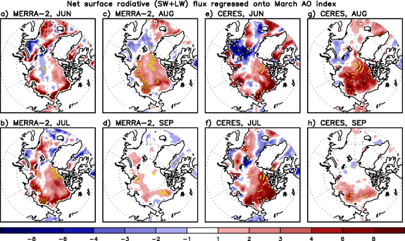
Figure 5. (a)–(d) Time evolution (June to September) of the total net (shortwave + longwave) radiative flux anomaly at surface from MERRA-2 regressed onto the March AO index in the 21st century (2000–2021). (e)–(h) Same as (a)–(d) but for the radiative flux anomalies from CERES-EBAF. Unit is W m−2. Stippling represents the grid points where anomaly is significant at 95% confidence.
Download figure:
Standard image High-resolution imageIt has been understood that the shortwave radiative flux can contribute significantly to the surface energy budget in summer (Persson et al 2002, Döscher et al 2014). By further separating the total radiative flux into shortwave and longwave flux, we are interested in identifying how the lagged response of shortwave flux to the March AO evolves with time over the entire course of boreal summer. The net shortwave flux from June to September explains that the positive anomaly, indicative of weak shortwave reflectivity to solar insolation, is especially stronger along the LECB region (figures 6(a)–(d)), where more sea ice decrease is found in figure 2. This positive anomaly is largest in that region in June and tends to weaken gradually with time (figures 6(c) and (d)). Nonetheless, spatial pattern in figures 6(a)–(d) indicates that the impact of positive AO in March is still active in August and September, contributing to continued surface warming and sea ice decrease along the LECB region.
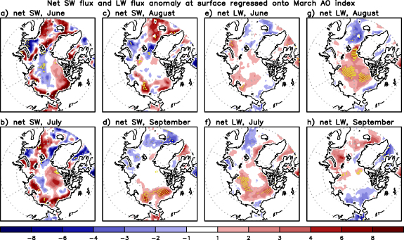
Figure 6. (a)–(d) Time evolution (June to September) of the net downward shortwave flux at surface over ocean regressed onto the March AO index in the 21st century (2000–2021). Unit is W m−2. (e)–(h) Same as (a)–(d) but for net downward longwave flux. Stippling represents the grid points where anomaly is significant at 95% confidence.
Download figure:
Standard image High-resolution imageIn contrast, the longwave flux plays as a moderate contributor to surface warming in summer. Figures 6(e)–(h) exhibit positive anomalies in the Arctic, but with smaller amplitude than the net shortwave flux. In addition, while the net shortwave flux contributes to warming close to the coastal area of LECB, the positive net longwave flux anomaly is seen over inner part of the Arctic Ocean clearly in July and August (figures 6(f) and (g)). Distribution of this positive anomaly is shown to resemble well the distribution of positive total cloud fraction anomaly in the Arctic (figure S4). Compared to the net shortwave/longwave fluxes, the amplitude of latent heat and sensible heat fluxes are relatively smaller (figure S5), indicating that the surface warming/cooling is more contributed by net radiative fluxes.
More absorption of shortwave radiation (figure 6), surface warming (figure 4), and sea ice decrease (figure 2) during the melt season raises an interesting question about their physical connections to atmospheric circulation. Low-level (925 hPa) wind and SLP anomalies regressed onto the March AO elucidate their time evolution from March through September (figure 7). Figure 7(a) for March represents the typical pressure/circulation pattern associated with the positive phase of the AO. This spatial structure weakens in April. Subsequently, the positive SLP anomaly in conjunction with anticyclonic circulation anomaly develops over the Arctic starting in May (figures 7(b)–(g)). This pattern continues to enhance forming the well-established spatial structure of anticyclonic circulation centered over Greenland and North Pole (Wang et al 2009, Ogi and Wallace 2012). It is also clear that the SLP anomaly over the sub-polar continents is near zero or negative in summer (Screen et al 2011), similar to the negative phase of the AO (figures 7(d)–(f)). Low-level wind surrounding the positive SLP anomaly blows from the west of Greenland toward the Arctic Ocean. The anticyclonic circulation anomaly also forms the northerly flow that blows from the North Pole to the Fram Strait. West and east of Greenland is characterized by warm and cold condition, respectively, due to this circulation anomaly observed in May through August. More absorption of solar radiation, surface warming and sea ice decrease described earlier are located along the northern flank of positive SLP and anticyclonic circulation anomaly. In contrast, less absorption of solar radiation, surface cooling and sea ice increase are located over the northeast of Greenland, where the northerly flow is predominant.

Figure 7. Same as figure 4 but for sea level pressure anomaly (shaded) and horizontal circulation anomaly at 925 hPa level (vectors). Units of the sea level pressure and wind are hPa and m s−1, respectively.
Download figure:
Standard image High-resolution image
The SLP and circulation in earlier months (March and April) are nearly opposite to the features seen in May through August, causing warming over east of Greenland (figures 4(a) and (b)). It is suggested that strong negative SLP anomaly and cyclonic circulation anomaly in accordance with the positive AO in March (figure 7(a)) could induce more cloudiness and downward longwave flux over the Arctic Ocean. This can drive relatively stronger warming in March than in April in the Arctic as we find that monthly difference in figure 4.
More importantly, it is worth noting that these SLP and circulation anomalies remarkably differ from those in the late 20th century (figure S6). Comparison between figures 7 and S6 demonstrates that, in the late 20th century, the SLP and circulation in summer does not reflect well the reversal of the March AO phase. As a result, the Canada Basin is not characterized by the strong southerly flows passing through the west of Greenland that is found in the 21st century. It in turn indicates unfavorable condition for sea ice decrease in this region in the late 20th century as it was discussed earlier in figure 3.
4. Conclusion and discussion
The impact of the March AO on the Arctic sea ice in the following summer is investigated in this study. While earlier studies average over winter or winter–spring to investigate the cold season AO impact on the interannual variation of the summertime sea ice, this study clearly found that the March AO is more highly correlated with the summertime sea ice than the AOs in the other boreal winter months or in spring (e.g. April and May). Specifically, a significant negative relationship of the AO between March and summer is identified, with the maximum anticorrelation in August. Time evolution of surface warming from surface energy budget, shortwave/longwave radiative flux, SLP and low-tropospheric circulation depict comprehensively how the AO phase in March gradually fades away and then transitions to the negative phase over the period from April to August. Anomalous sea ice distribution in each month is reasonably explained by time evolution of surface energy budget and SLP/circulation. Sea ice decrease enhances along the LECB region during the melt season in the event of positive AO in March, whereas the sea ice increases over the region to the northeast of Greenland. The sea ice decrease along the LECB region is found to be more active in the recent 21st century (2000–2021) than later part of the 20th century (1980–1999), due to the fact that sea ice is thinner and more susceptible to surface warming and sea ice motion (Maslanik et al 2007, Williams et al 2016, Gregory et al 2022). Also, different atmospheric circulation response to the March AO between the 21st and 20th century yields the opposite sea ice anomaly between the two periods over the Canada Basin.
The strong anticorrelation of the AO between March and summer in this study is based on the NOAA index that focuses on the 1000 hPa geopotential height. Additionally, we compute our own AO index by applying the upper-level (250 hPa) MERRA-2 geopotential height to verify that the strong anticorrelation of the AO between March and the following summer is robust. We first find that this AO index is highly correlated with the NOAA index (0.93 in March and 0.66 in summer). Time-lagged correlations of the AO time series between March and the subsequent months clarify a dramatic growth of negative correlation with time reaching the peak in August (figure S7(d)), identical to the feature based on the NOAA index.
Arctic sea ice historic record in peak melt season (e.g. September) indicates that the years characterized by significant melting are 2007, 2008, 2011, 2012, 2015, 2016, 2019 and 2020 (https://nsidc.org/arcticseaicenews/charctic-interactive-sea-ice-graph/). The March AO index in those years was strongly in positive, generally a good agreement with the findings in this study. On the other hand, 2013 and 2018 are the years that experience more sea ice extent in melt season than the other years. The March AO in those two years was in negative phase.
Our further interest is whether more sea ice loss than average over the LECB region occurs only when the AO is in positive phase with no exception in the preceding cold season. Despite the negative AO phase in early 2010, atmospheric circulation, specifically the Beaufort Gyre responsible for ice transport and thickening of ice in the Canada Basin was not so enhanced in 2010, compared to the mean anomaly pattern based on negative AO events (Stroeve et al 2011), resulting in the above average sea ice loss in the boreal summer. Please note, however, that this negative sea ice anomaly is not greater than that observed in the subsequent strong melt years in 2010s. The case in 2010 suggests that the atmospheric process could be occasionally exceptional causing more sea ice decrease than average even if the AO is not in the positive phase in the preceding winter. This study also suggests that, while a very interesting connection between the March AO and summertime sea ice is found, fully-coupled simulations with more complex representations of sea ice and snow on the ice are needed to more directly test these connections.
Acknowledgments
This research was supported by NASA Sun-Climate research fund to Goddard Space Flight Center, Award Number 509496.02.03.01.17.04.
Data availability statement
The monthly AO index from NOAA is downloaded from www.cpc.ncep.noaa.gov/products/precip/CWlink/daily_ao_index/ao.shtml. MERRA-2 data are downloaded from NASA's EarthData website https://disc.gsfc.nasa.gov/datasets/. The sea ice data from the NSIDC is downloaded from https://nsidc.org/data/G10010. The CERES-EBAF radiative fluxes are downloaded from https://asdc.larc.nasa.gov/project/CERES/CERES_EBAF_Edition4.1.
The data that support the findings of this study are available upon reasonable request from the authors.
Conflict of interest
The authors declare no conflict of interest
Supplementary data (1.2 MB PDF)